This paper is available on arxiv under CC 4.0 license.
Authors:
(1) Ali Ghanbari, Dept. of Computer Science, Iowa State University;
(2) Deepak-George Thomas, Dept. of Computer Science, Iowa State University;
(3) Muhammad Arbab Arshad, Dept. of Computer Science, Iowa State University;
(4) Hridesh Rajan, Dept. of Computer Science, Iowa State University.
Table of Links
- Abstract & Introduction
- Background
- Motivating Example
- Proposed Approach
- Supported DNN Bugs
- Evaluation
- Threats to Validity
- Related Work
- Conclusion, Acknowledgments & References
II. BACKGROUND
A. Mutation Analysis
Mutation analysis [18], is a program analysis method for assessing the quality of the test suite. It involves generating a pool of program variants, i.e., mutants, by systematically mutating program elements, e.g., replacing an arithmetic operator with another, and running the test suite against the mutants to check if the output of the mutated program is different from that of the original one; if different, the mutant is marked as killed, otherwise as survived. A mutant might survive because it is semantically equivalent to the original program, hence the name equivalent mutant. Test suite quality is assessed by computing a mutation score for the test suite, which is the ratio of killed mutants over the non-equivalent survived mutants. Mutation score indicates how good a test suite is in detecting real bugs [37]. In addition to its original use, mutation analysis has been used for many other purposes [38], such as fault localization [16], [17], automated program repair [39], [40], test generation [41], [42] and prioritization [43], program verification [44], [45], etc.
B. Mutation-based Fault Localization
Mutation-based fault localization (MBFL) uses mutation analysis to find bugs. In this section, we review two major approaches to MBFL, namely Metallaxis [30] and MUSE [17]. Both of these approaches are implemented in deepmufl. The reader is referred to the original papers [30], [17] for examples explicating the rationale behind each approach.
1) Metallaxis: Metallaxis [30] posits that mutants generated by mutating the same program element are likely to exhibit similar behaviors and mutants generated by mutating different program elements are likely to exhibit different behaviors. Since a fault itself can also be viewed as a mutant, it is expected to behave similar to other mutants generated by mutating that same buggy program element and can be located by examining the mutants based on this heuristic. Metallaxis assumes that the mutants impacting the test outputs, or their error messages, e.g., stack trace, as impacting the tests. Thus, mutants impacting failing test cases might indicate that their corresponding code elements is the root cause of the test failures, while mutants impacting passing test cases might indicate that their corresponding code elements are correct.
Once the number of impacted passing and failing test cases are calculated, Metallaxis uses a fault localization formula to calculate suspiciousness values for each element.
Metallaxis fault localization formula can be viewed as an extension to that of spectrum-based fault localization, by treating all mutants impacting the tests as covered elements while the others as uncovered elements. Specifically, the maximum suspiciousness value of the mutants of a corresponding code element is returned as the suspiciousness value of the code element. More concretely, assuming we are using SBI formula [46], suspiciousness value for a program element e, denoted s(e), is calculated as follows.

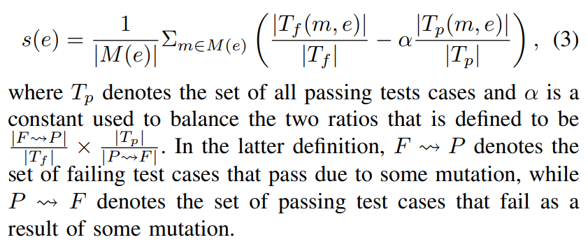
where M(e) denotes the set of all mutants targeting program element e, Tf (m, e) is the set of failing test cases that are impacted by the mutant m, while Tp(m, e) denotes the set of passing test cases that are impacted by m. In this definition, and in the rest of the paper, the notation | · | represents the size of a set. Alternatively, had we used Ochiai [47], Metallaxis suspiciousness formula would be modified as follows.

where Tf denotes the set of all failing tests cases.
2) MUSE: MUSE [17] is based on the assumption that mutating a faulty program element is likely to impact more failed test cases than passing test cases by “fixing” it, while mutating a correct program element is likely to impact more passing test cases than failing test cases by breaking it. The notion of “impacting test cases” in MUSE, unlike Metallaxis, is more rigid, in that it refers to making passing test cases fail, vice versa. Once the number of impacted failing and passing test cases are identified, suspiciousness values can be calculated using the following formula.

C. Deep Neural Networks
A neural network is intended to compute a function of the form R m −→ R n, where m, n are positive integers. A neural network is often represented as a weighted directed acyclic graph arranged in layers of three types, i.e., input layer, one or more hidden layers, and an output layer. Input and output layers output linear combination of their inputs, while hidden layers can be viewed as more complex computational units, e.g., a non-linear unit, convolutional unit, or a batch normalization unit. A non-linear unit is composed of neurons, functions applying a non-linear activation function, e.g., rectified linear unit (ReLU), tanh, or sigmoid, on the weighted sum of their inputs. A convolutional layer, calculates the convolution between the vector of the values obtained from the previous layer and a learned kernel matrix. Lastly, a batch normalization layer, normalizes the vector of values obtained from the previous layer via centering or re-scaling. A neural network with two or more hidden layers is referred to as a deep neural network (DNN).

