This paper is available on arxiv under CC 4.0 license.
Authors:
(1) Vianney Brouard, ENS de Lyon, UMPA, CNRS UMR 5669, 46 All´ee d’Italie, 69364 Lyon Cedex 07, France; E-mail: [email protected].
Table of Links
- Abstract & Introduction and presentation of the model
- Main results and biological interpretation
- First-order asymptotics of the mutant sub-populations for an infinite mono-directional grap
- First-order asymptotics of the mutant sub-populations for a general finite trait space (Theorem 2.1)
- Convergence for the stochastic exponents (Theorem 2.2)
- Acknowledgements & References
2 Main results and biological interpretation
In Subsection 2.1 the first-order asymptotics of the size of all the mutant sub-populations in the timescales (3) and (4) are given under the non-increasing growth rate condition (5). In Subsection 2.2 the asymptotic result on the stochastic exponent of all the mutant sub-populations are given without any assumption on the growth rate function λ. In each subsection, biological interpretations of the results are made.
2.1 First-order asymptotics of the mutant sub-population sizes under nonincreasing growth rate condition
In this subsection assume that (V, E, L) satisfies the non-increasing growth rate graph condition of Equation (5).
Heuristics:
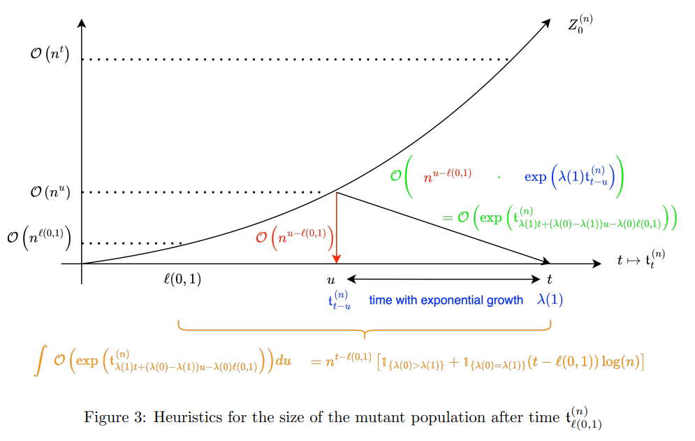
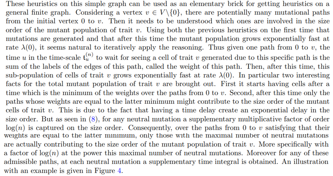
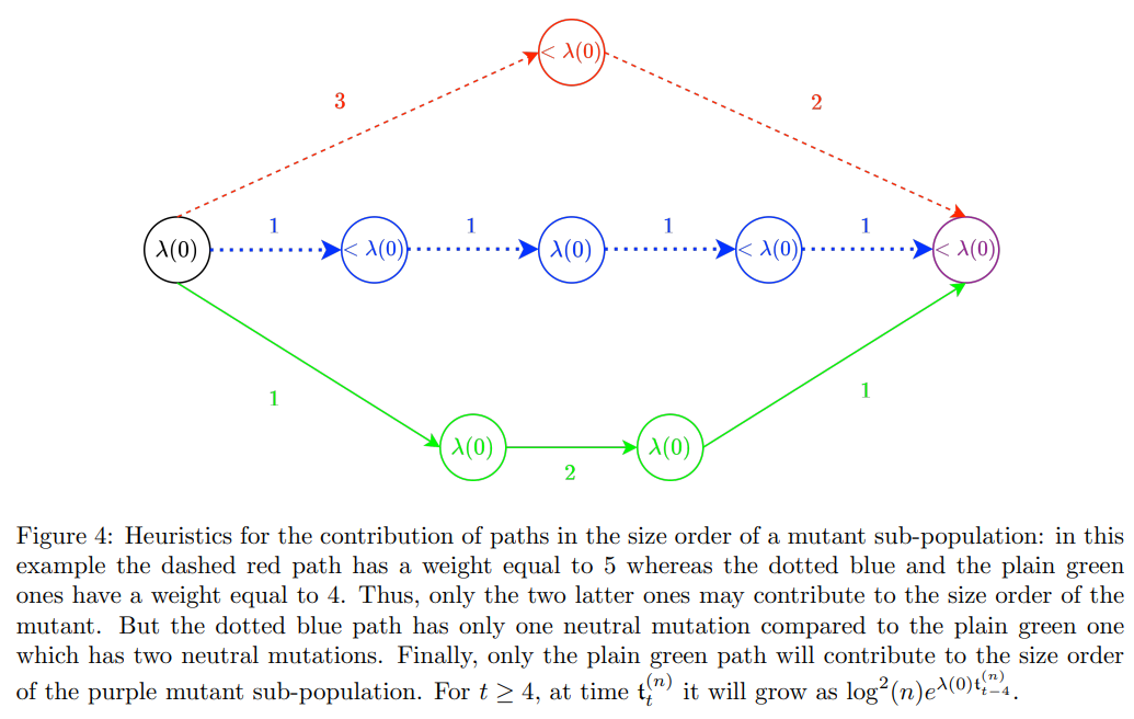
The next definitions, notations and results are first motivated using some heuristics for the simplest graph that one can think of, i.e. a wild-type and a mutant population where only mutations from wild-type to mutant cells are considered. More precisely (V, E, L) = ({0, 1}, {(0, 1)}, {ℓ(0, 1)}) as in Figure 1.
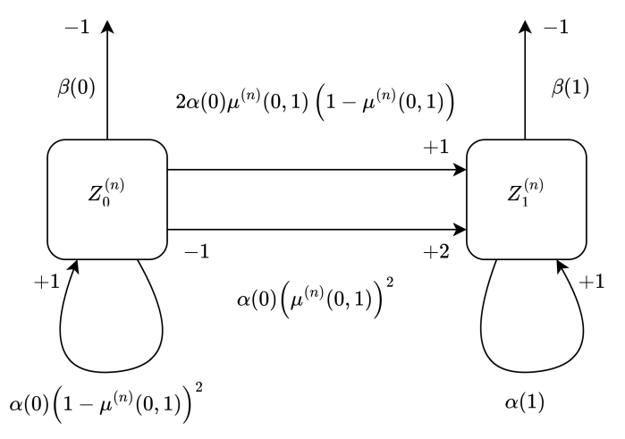
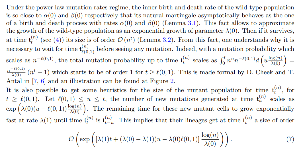
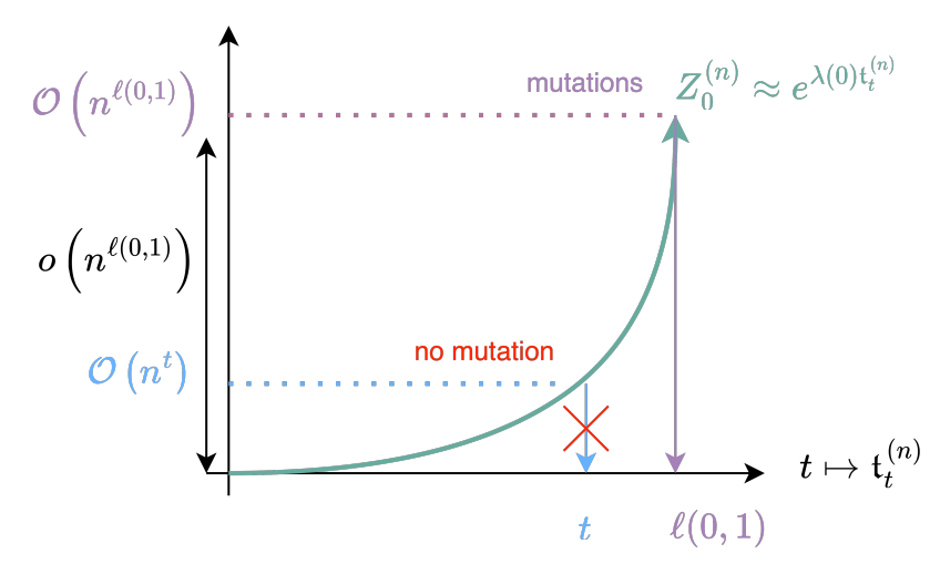
Then two scenari are possible:



Notations:
Now the natural definitions issued from these heuristics are formally made before giving the results.
Definition 2.1. (Deleterious and neutral vertices)
A vertex v ∈ V satisfying λ(v) = λ(0), respectively λ(v) < λ(0), is called a neutral, respectively deleterious, vertex.
Remark 2.1. In the previous definition the neutral or deleterious denomination of a mutation originates from the comparison of its inner growth rate to the growth rate of the wild-type population. But one could imagine a mutation from a vertex v to a vertex u satisfying λ(v) < λ(u) ≤ λ(0). This mutation should theoretically be called selective but in the previous definition it is actually called neutral or deleterious (depending on the value of λ(u) compared to λ(0)). This nomenclature emerges from the fact that under Assumption (5) any mutant population grows exponentially fast at rate λ(0), as seen in the previous heuristics. Hence it legitimates the previous definition.
Definition 2.2. (Path on the graph)
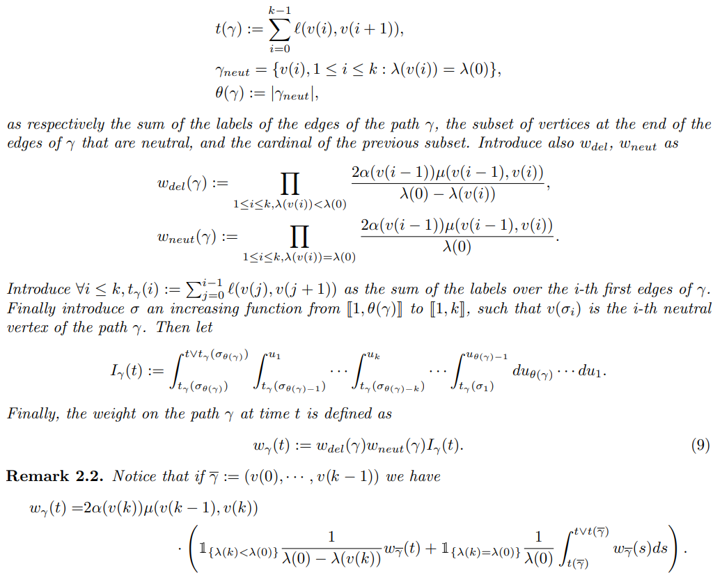
γ = (v(0), · · · , v(k)) is said to be the path on the graph (V, E) linking v(0) to v(k) by using the edges (v(i), v(i + 1)) if for all 0 ≤ i ≤ k, v(i) ∈ V and ∀0 ≤ i ≤ k − 1,(v(i), v(i + 1)) ∈ E. For a path γ = (v(0), v(1), · · · v(k)) on (V, E, L) define
Definition 2.3. (Admissible paths)
For all v ∈ V denote by P(v) the set of all paths γ on (V, E) linking the vertex 0 to the vertex v. Define also
t(v) := min{t(γ), ∀γ ∈ P(v)},
θ(v) := max {θ(γ), ∀γ ∈ P(v), t(γ) = t(v)} ,
A(v) := {γ ∈ P(v) : t(γ) = t(v) and θ(γ) = θ(v)}.
Remark 2.3. In the previous definition A(v) is called the set of admissible paths because as seen in the heuristics, only paths belonging to A(v) are contributing to the growth dynamics of the mutant cells of trait v. This is made formal in Theorem 2.1.
Definition 2.4. (Weight of a vertex)
The weight of a vertex v ∈ V \{0} at time t is defined as


Results:
Now the more refined result under Assumption (5) can formally be stated.
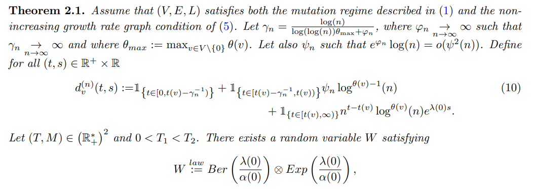
such that for all v ∈ V \{0} we obtain the following results for the different time-scales:
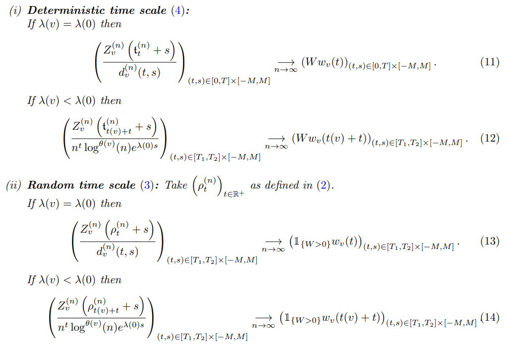
Using the mathematical definition of the model given in Section 4, see (78) and (79), the above convergences are obtained in probability in the adequate L∞-spaces. For any other mathematical description, the convergences are at least in distribution in D ([0, T] × [−M, M]) for Equation (11) and in D ([T1, T2] × [−M, M]) for Equations (12), (13) and (14).
The proof of Theorem 2.1 is based on a martingale approach using Doob’s and Maximal Inequalities. The first step involves the control of the growth of the lineage of wild-type cells issued from the initial cell both for the deterministic and random time-scales (4) and (3) (Lemma 3.1 and 3.2). Then for any vertex v ∈ V \{0}, potentially many mutational paths on the graph (V, E) can start from 0 and lead to v. The contribution on the first-order asymptotics of the mutant sub-population of trait v for any of these paths needs to be understood. The proof is then done in 2 steps. The first one consists in considering an infinite mono-directional graph under Assumption (5) and in obtaining the result for this particular graph, see Section 3. Doing the first step for an infinite graph allows in particular to deal with the cycles (backward mutations for instance) for a general finite graph. The second step consists in discriminating among all the paths from the initial vertex 0 to v the ones that do not contribute to the first-order asymptotics of the mutant sub-population of trait v, see Section 4.

(ii) The random variable W is explicitly defined as the almost sure limit of the natural positive martingale associated to a specific birth and death branching process with rates α(0) and β(0), see (81). The martingale associated to the lineage of wild-type cells issued from the initial cell is shown to behave as the one associated to the latter birth and death branching process (Lemma 4.1). Thus W quantifies the randomness of this lineage over the long time. Due to the power law mutation rates regime mutations arise after a long time such that the stochasticity of this lineage is already given by W. Notice that under Assumption (5) the randomness in the first-order asymptotics of any mutant sub-population is summed up in W. Meaning that the stochasticity of these sub-populations are driven more by the stochasticity in the growth of the wild-type sub-population than by both the randomness in the mutational process and the randomness of any lineages of mutant cells.
(iii) It seems more than natural not to obtain such a result when considering selective mutation (λ(v) > λ(0)). Indeed, a selective mutation would mean that any time advantage is an advantage into growth. Thus the stochasticity of the mutational process can not be ignored as well as the one of the lineages of mutant cells. Hence hoping to control the stochasticity of the mutant population controlling only the randomness of the wild-type population and not the randomness of the mutational process as well as the one of the lineages of the mutant cells is vain. Meaning that using a martingale approach to get the first-order asymptotics can not be successful for a selective mutation. Nevertheless looking at the stochastic exponent (6) the martingale approach allows to get convergence results given in Theorem 2.2.
(iv) In view of Theorem 2.1, the mathematical definition of neutral mutation λ(v) = λ(0) is well understood instead of the more restrictive but biologically more meaningful condition α(v) = α(0) and β(v) = β(0). Indeed, taking the growth rate λ(v) equal to λ(0) when changing birth and death rates α(v) and β(v) modify the distribution of any lineage of mutant cells. Consequently one could naturally believe that it should impact the stochasticity of the size order of the mutant population. This is not the case, the randomness on the first asymptotic order is fully summed up by W. Hence it is fully consistent with getting for the neutral assumption only a condition on the growth rate function instead of on the birth and death rates.
(v) Considering the time-scale t (n) t notice that the result slightly differs depending on whether the vertex is neutral or deleterious. Indeed, when looking at the asymptotic behavior for a deleterious vertex v our result is true strictly after time t(v), whereas in the case of a neutral vertex all the trajectory from the initial time can be dealt with. Mathematically, this difference originates from the supplementary multiplicative log(n) factor in the first asymptotic order when considering a neutral mutation. It allows to control the quadratic variation at time t(v) for the martingale associated to the mutant population.
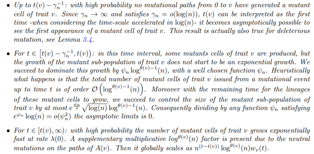
Then exactly three different regimes are obtained, see (10) and (11) :

2.2 Result for a general finite oriented labeled graph
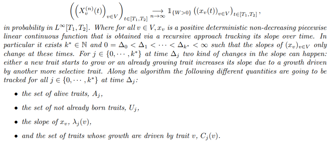
This subsection is free from the non-increasing growth rate condition of Equation (5). Without this condition, the martingale approach fails in order to get the first-order asymptotics off all the mutant sub-populations. But, the stochastic exponent, as defined in (6), off all the mutant sub-populations can be uniformly tracked over time. In particular, we show that the limits are positive deterministic non-decreasing piecewise linear continuous functions. Such limits are defined via a recursive algorithm tracking their slopes over time. More precisely, we show that the slopes can only increase and take values on the set of the growth rates. Two different kinds of updates can be made. The first one is when a non-already born trait becomes alive and take the slope which is the maximum between its inner growth rate and the slope of the sub-population that is giving birth to it. The second one is when an already born trait changes it slope to increase it because another born trait among its upcoming neighbors with a higher slope has reached the typical size allowing it to now drive the trait in question, and consequently giving it its slope. This heuristic is made formal in the following theorem. The complexity of such an algorithm comes from the trait structure which is a general finite trait space. On a mono-directional one, this algorithm would be much easier. In particular, at the same time, the two kinds of event can happen.
Theorem 2.2. For all v ∈ V define

Then we have for all 0 < T1 < T2,
Initialisation: Set A0 = {0}, U0 = V \{0} and for all v ∈ V
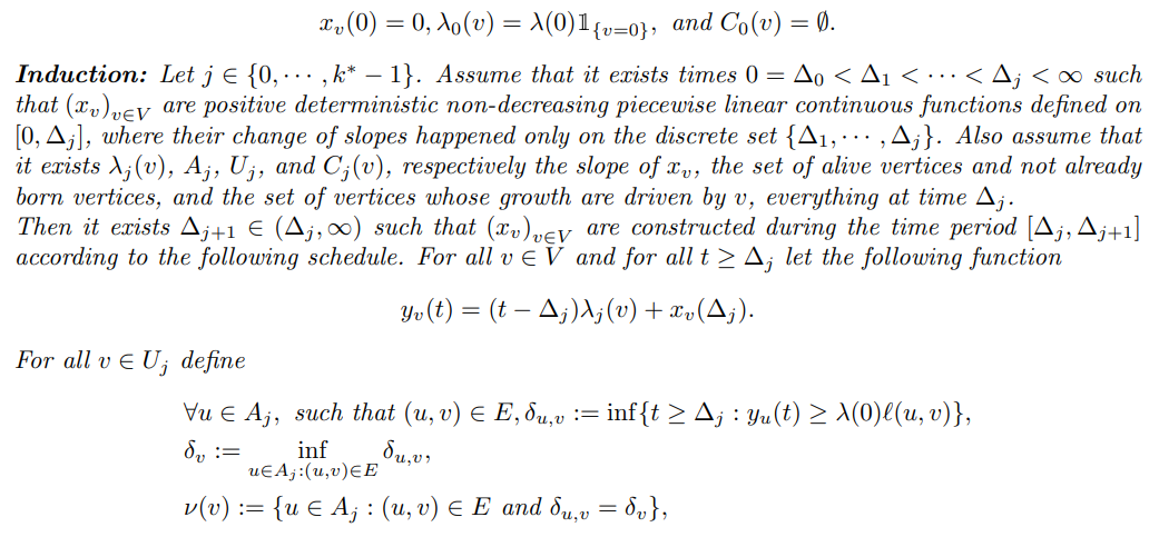
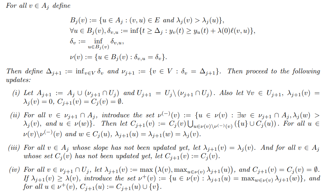
For any other mathematical description as the one given in Section 4, see (78) and (79), the convergences are at least in distribution in D ([T1, T2]).
The proof of this theorem is given in Section 5. It is heavily based on the proofs of [13], where we exploit the stochastic construction of such a model, given in the beginning of Section 4, to adapt the proofs of the previous article to the situation of the present work. For that reason, we introduce lemmas and explain in the proofs how the adaptations from the proofs of [13] are made, without reproving them. This theorem is the counterpart of the study made in [8] in the case of branching sub-populations, instead of having competition between sub-populations. One difference is that the power law mutation rates regime is a bit more general in the present work, allowing each mutation probabilities to scale differently. But, the result in [8] can be adapted with this more general regime, as mentioned by the authors.
